

Split your work
Working with a monolithic 2000-line script can be overwhelming and inefficient 😱.
This lesson delves into the drawbacks of such an approach and offers practical strategies for dividing your work into manageable, coherent segments.
Too long is too long
I am sure it already happened to you.
You write some code to analyse a dataset. It triggers some new questions. So you add some more code to understand. And so on!
You end up with a 2000 lines long file that takes 35 minutes to run from start to end.
This is annoying!
❌ Slow: when you open R again to modify the end of your script, you have to run the beginning again!
❌ Hard to maintain: navigating a 2000 lines long file is not fun at all.
❌ Bad for collaboration: if you are several people working on the same massive file, it is very likely that you get conflicts.
So. How can you do?
➡️ You have to modularize your code.
Modular programming is a design technique that involves separating a program into distinct modules that can be developed, tested, and debugged independently of each other.
And there are 3 main ways to do so:
1️⃣ Use Functions. Source() them.
In the previous lesson we saw how to avoid duplication in code by using functions.
If those functions are big, it is a good practice to isolate them in another file.
For instance, you can create a file called functions.R and write your functions in it.
Then, in your main analysis.R file, you can run source(functions.R). This will make the functions defined in functions.R available!
Let's try it!
penguin project in R Studio. Create a new file in the R directory called functions.RCopy the create_scatterplot() function we built in the previous lesson.
In the analysis.R file, source() the functions.R script and use the function!
2️⃣ Split your analysis in several steps
Let's say the first part of your work involves exploratory analysis. The second step focuses on creating a statistical model to enable future predictions.
In this context, it's logical to organize your scripts accordingly. Start with a script named 01_exploratory_analysis.R for the initial analysis, followed by 02_modeling.R for the modeling phase.
This approach significantly enhances readability, execution, and maintenance of your code.
Our analysis.R is rather small for now. But we'll see later in this course how to split it.
3️⃣ Create intermediary dataset
The first step in data analysis typically involves loading, cleaning, and wrangling a dataset. This process results in a refined dataset, often enriched with additional columns, primed for visualization and analysis.
This initial stage may require significant computational resources. Hence, it's a recommended practice to isolate this step in a separate script, allowing the script to output the cleaned dataset. This strategy prevents the need to re-run this computationally intensive step during subsequent phases of the analysis.
R provides the efficient .rds format for storing R objects. This format can be conveniently used to save and subsequently load data using the saveRDS() and readRDS() functions. The .rds format is lightweight and fast, offering a more efficient alternative to traditional CSV files.
17kb for the penguin .xlsx file. 3kb for the .rds equivalent! 🔥
01_load_clean_data.R.In this file, write some code that loads the penguin dataset, removes row 23 and 48, and save the result as clean_data.rds in the input folder.
In the analysis.R file, load the clean_data.rds content.
Project organization
We are now reaching a pretty solid project organization pattern:
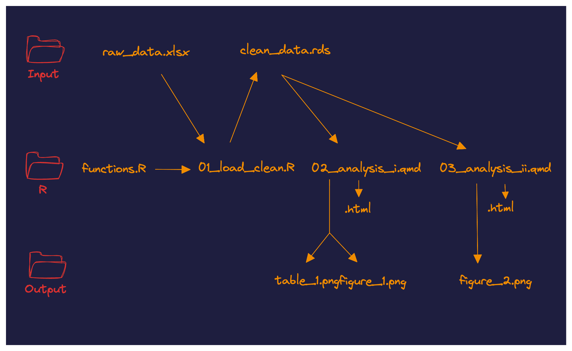
Everything starts with the raw dataset raw_data.xlsx.
This file is read by the first step of our pipeline: 01_load_clean.R, that can potentially use functions stored in functions.R. The script outputs a clean clean_data.rds file that can then be read in the subsequent parts of the analysis.
Of course you do not have to follow this exact structure. But hopefully this can be a good inspiration.